谱减法（一）

import librosa
from librosa.core.spectrum import amplitude_to_db
import numpy as np
import soundfile as sf
import matplotlib.pyplot as plt

if __name__ == "__main__":
    clean_wav_file = "sf1_cln.wav"
    clean,fs = librosa.load(clean_wav_file, sr=None)
    print(fs)

    noisy_wav_file = "sf1_n0L.wav"
    noisy,fs = librosa.load(noisy_wav_file, sr=None)

    # compute the STFT of the noisy signals
    noisy_stft = librosa.stft(noisy, n_fft=256, hop_length=128, win_length=256)     # D x T
    D,T = np.shape(noisy_stft)
    Mag_noisy = np.abs(noisy_stft)
    Phase_noisy = np.angle(noisy_stft)
    power_noisy = Mag_noisy**2
    print(fs)
    # estimate the noise power
    Mag_noisy = np.mean(np.abs(noisy_stft[:,:30]), axis=1, keepdims=True)
    power_noise = Mag_noisy**2
    power_noise = np.tile(power_noise, (1,T))

    #subtract the noise power from the noisy power   
    power_enhanc = power_noisy - power_noise
    power_enhanc[power_enhanc < 0] = 0
    Mag_enhanc = np.sqrt(power_enhanc)

    #subtract the noise amplitude from the noisy amplitude
    # Mag_enhanc = np.sqrt(power_noisy) - np.sqrt(power_noise)
    # Mag_enhanc[Mag_enhanc < 0] = 0

    # reconstruct the enhanced signal
    enhanc_stft = Mag_enhanc * np.exp(1j*Phase_noisy)
    enhanc = librosa.istft(enhanc_stft, hop_length=128,win_length=256)
    sf.write("enhanc.wav", enhanc, fs)
    print(fs)

    # plot the spectrograms
    plt.subplot(3,1,1)
    plt.specgram(clean, NFFT=256, Fs=fs)
    plt.xlabel("clean specgram")
    plt.subplot(3,1,2)
    plt.specgram(noisy, NFFT=256, Fs=fs)
    plt.xlabel("noisy specgram")
    plt.subplot(3,1,3)
    plt.specgram(enhanc, NFFT=256, Fs=fs)
    plt.xlabel("enhanc specgram")
    plt.show()

    plt.imshow(librosa.amplitude_to_db(np.abs(Mag_enhanc), ref=np.max), origin='lower')
    plt.show()

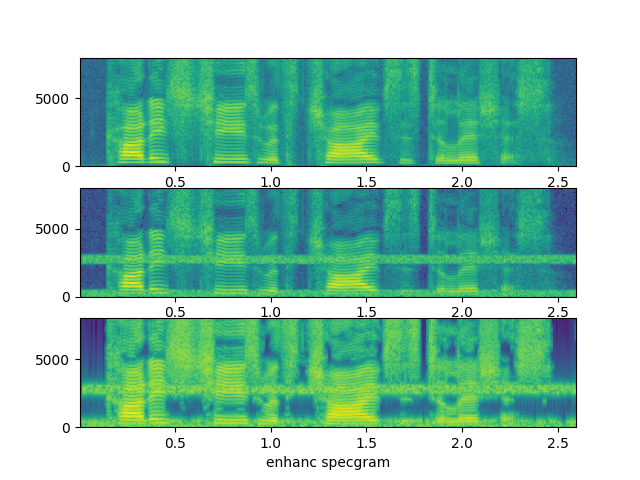
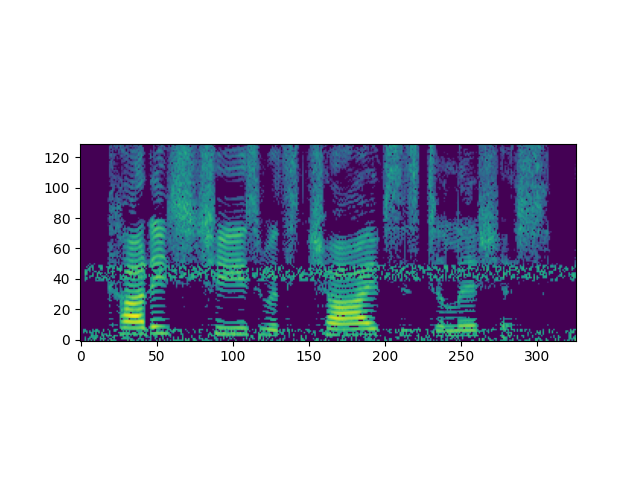
最上面是干净语音的频谱，中间是加噪后的频谱，下面是通过谱减法后的频谱。气质，最下面通过谱减后仍存在噪声，我们称之为噪声残留，也叫做音乐噪声。其与频谱泄露有关。